sampling and aliasing
Table of Contents
模拟信号(analog signal)和数字信号(digital signal)是两种不同类型的信号,在电子通讯和 信号处理领域中有重要作用。
模拟信号是连续变化的信号,它的取值是在一定范围可以无限细分的(连续型变量)。例如声音波形。
数字信号是离散的信号,是对模拟信号进行离散化(采样和量化)得到的。进行这种离散化操作的叫 做模数转换器(ADC),转成数字信号后方便存储和传输,但利用这些数字信号时通常需要再将它们转 换为模拟信号(通过数模转换器,DAC),因为人类不像计算机,不能直接处理0/1信号,只能接收模 拟信号。(人的耳朵解析的是模拟信号,恐怕还没人练就听一串01组成的数字就能听出那是贝多芬的 第九交响曲的本领。)
#
混叠现象(Aliasing)
混叠(Alias)现象的产生是由于采样定理(也称为奈奎斯特定理)未被满足。奈奎斯特定理指出, 为了避免混叠,采样频率必须至少是信号中最高频信号频率的两倍。如果信号频率高于采样频率的一 半,就会出现混叠现象。也就是:它发生在信号的采样频率不足以表示原始信号中的所有频率成分时:
- 当信号中某些组分的信号频率高于采样频率的一半(也称为:折叠频率)时,高频部分会被错误的 解析成低频信号,这就导致频谱中出现虚假的频率成分(本是高频的,被折叠为低频的)。
- 由于折叠频率的存在,信号频谱中部分频率被重叠,导致信息丢失和失真。
##
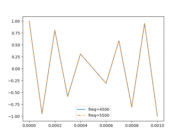
采样采样,越采越像
framerate = 10000  # 采样频率

# 构建原始信号,频率:4500
signal = thinkdsp.CosSignal(4500)
duration = signal.period*5
# 对原始信号进行采样
segment = signal.make_wave(duration, framerate=framerate)
segment.plot(label="freq=4500")

# 构建原始信号,频率:5500
signal = thinkdsp.CosSignal(5500)
# 对原始信号进行采样
segment = signal.make_wave(duration, framerate=framerate)
segment.plot(linestyle="-.", label="freq=5500")

plt.legend()
##
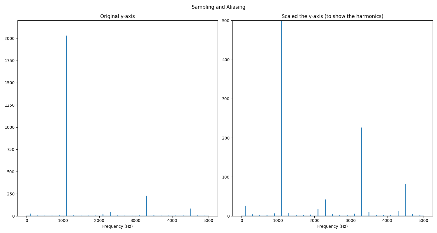
混叠的频率
下面是一个三角形信号(频率为1100)的频谱图,注意其谐波(harmonics)应该是基频 (fundamental frequency)的奇数倍(如 3300,5500,7700,9900,12100等等),但是,并非完 全如此,第三个谐波出现在4500,而第四个则在2300,认真看右边的y轴放大图,第五个出现在100的 位置,而第六个呢(在2100的位置)。啥情况?!
这就是混叠现象。采样频率为10k,折叠频率=$\frac{1000}{2}=5000$,当信号中频率高于5000的, 会被“折叠”(折回来,回到小于折叠频率的范围内)。所以,频率为5500的谐波被折叠到4500的位置, 同理,频率为7700的谐波被折叠到2300的位置,以此类推(镜像中心就是5000的位置)。
就这样,原本的三角波形模拟信号经过这个采样得到的数字信号,再重新转换为模拟信号时,已失真。
fig, axs = plt.subplots(1, 2, figsize=(15, 8))

signal = TriangleSignal(1100)
segment = signal.make_wave(duration=0.5, framerate=10000)
spectrum = segment.make_spectrum()
axs[0].plot(spectrum.fs, spectrum.hs)
axs[0].set_ylim(0, 2200)
axs[0].set_xlabel('Frequency (Hz)')
axs[0].set_title('Original y-axis')

signal = TriangleSignal(1100)
segment = signal.make_wave(duration=0.5, framerate=10000)
spectrum = segment.make_spectrum()
axs[1].plot(spectrum.fs, spectrum.hs)
axs[1].set_ylim(0, 500)
decorate(xlabel='Frequency (Hz)')
decorate(title='Scaled the y-axis (to show the harmonics)')

plt.suptitle('Sampling and Aliasing')
plt.tight_layout()
#
频谱是怎么计算得到的
频谱图实际上就是以频率(frequency)为横轴,幅度(amplitude)为纵轴的图。
那么,信号中的频率及其幅度又是怎么算出来的?快速傅里叶转换(FFT)。
def plot(self, high=None, **options):
    """Plots amplitude vs frequency.

    Note: if this is a full spectrum, it ignores low and high

    high: frequency to cut off at
    """
    if self.full:
        fs, amps = self.render_full(high)
        plt.plot(fs, amps, **options)
    else:
        i = None if high is None else find_index(high, self.fs)
        plt.plot(self.fs[:i], self.amps[:i], **options)

def render_full(self, high=None):
    """Extracts amps and fs from a full spectrum.

    high: cutoff frequency

    returns: fs, amps
    """
    hs = np.fft.fftshift(self.hs)
    amps = np.abs(hs)
    fs = np.fft.fftshift(self.fs)
    i = 0 if high is None else find_index(-high, fs)
    j = None if high is None else find_index(high, fs) + 1
    return fs[i:j], amps[i:j]
##
DFT & FFT
快速回顾: 离散傅里叶转换(DFT)是一种数学思想(所有波可以由若干正余弦波叠加而成), 而快速傅里叶转换(FFT)是一种高效算法,用于实现离散傅里叶转换。
快速回顾2: 傅里叶级数是一种将周期函数(periodic function)分解为一系列正弦和余弦函数的无穷和的方法。 假设我们有一个周期为 $ T $ 的函数 $ f(t) $,它可以表示为如下的傅里叶级数:
$$ f(t) = \frac{a_0}{2} + \sum_{n=1}^{\infty} \left( a_n \cos\left(\frac{2\pi nt}{T}\right) + b_n \sin\left(\frac{2\pi nt}{T}\right) \right) $$
其中 $ a_0, a_n, b_n $ 是系数,它们可以通过函数 $ f(t) $ 的周期性质计算得到。
系数的计算公式为:
$$ \begin{align*}% align* 的 * 号用于阻止自动编号生成; hugo中要用 \\ 换行,第一个\为转义字符 a_0 &= \frac{1}{T} \int_{0}^{T} f(t) dt \\ a_n &= \frac{2}{T} \int_{0}^{T} f(t) \cos\left(\frac{2\pi nt}{T}\right) dt \\ b_n &= \frac{2}{T} \int_{0}^{T} f(t) \sin\left(\frac{2\pi nt}{T}\right) dt \end{align*} $$
这些系数描述了正弦和余弦函数的振幅和相位,它们决定了如何将原始函数 $ f(t) $ 分解成频率 为 $ \frac{n}{T} $ 的正弦和余弦函数的和。
from np.fft import rfft, rfftfreq

class Wave:

    # lots of other attrs, methods

    def make_spectrum(self):
        """
        self: Wave object
        """
        # n   : number of samples in the wave
        # d   : inverse of framerate, means the time between samples
        # hs  : a NumPy array of complex numbers that represents the amplitude and
        #       phase offset of each frequency component in the wave
        # fs  : an array that contains frequencies corresponding to the `hs`

        n = len(self.hs)
        d = 1 / self.framerate

        hs = rfft(self.ys)
        fs = rfftfreq(n, d)

        return Spectrum(hs, fs, self.framerate)