# Plain and Simple: IndexFlatL2

Given a set of vectors, we can index them using Faiss — then using another vector (the query vector), we search for the most similar vectors within the index. Now, Faiss not only allows us to build an index and search — but it also speeds up search times to ludicrous performance levels.

IndexFlatL2 measures the L2 (or Euclidean) distance between all given points between our query vector, and the vectors loaded into the index. It’s simple, very accurate, but not too fast.

Image credit: pinecone.io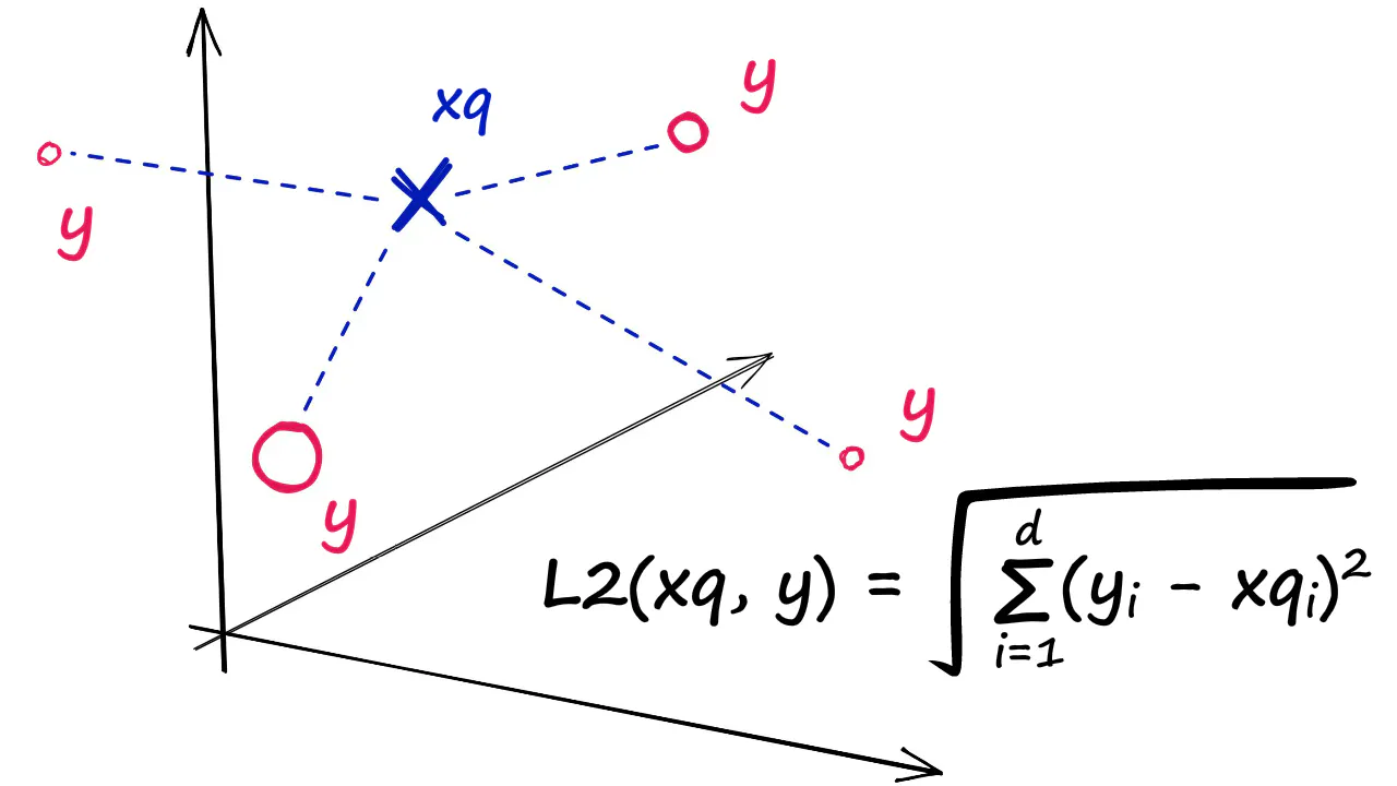

• IndexFlatL2: simple but not scalable
• Partitioning the index: for speed when scale up
• Quantization: for more speed

Image credit: pinecone.io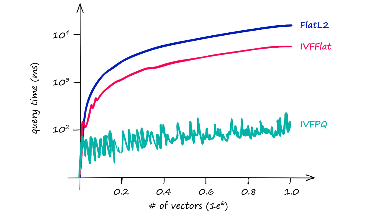

# Inverted File Index (IVF) index

The Inverted File Index (IVF) index consists of search scope reduction through clustering.

Inverted File Index (IVF) The IVF is simply a technique for pre-filtering the dataset so that you don’t have to do an exhaustive search of all of the vectors. It’s pretty straightforward–you cluster the dataset ahead of time with k-means clustering to produce a large number (e.g., 100) of dataset partitions. Then, at query time, you compare your query vector to the partition centroids to find, e.g., the 10 closest clusters, and then you search against only the vectors in those partitions.

Partitioning the index (clustering)

Faiss allows us to add multiple steps that can optimize our search using many different methods. A popular approach is to partition the index into Voronoi cells. We can imagine our vectors as each being contained within a Voronoi cell — when we introduce a new query vector, we first measure its distance between centroids, then restrict our search scope to that centroid’s cell. But there is a problem if our query vector lands near the edge of a cell — there’s a good chance that its closest other datapoint is contained within a neighboring cell.

what we can do to mitigate this issue and increase search-quality is increase an index parameter known as the nprobe value. With nprobe we can set the number of cells to search. I.e., Increasing nprobe increases our search scope.

Image credit: pinecone.io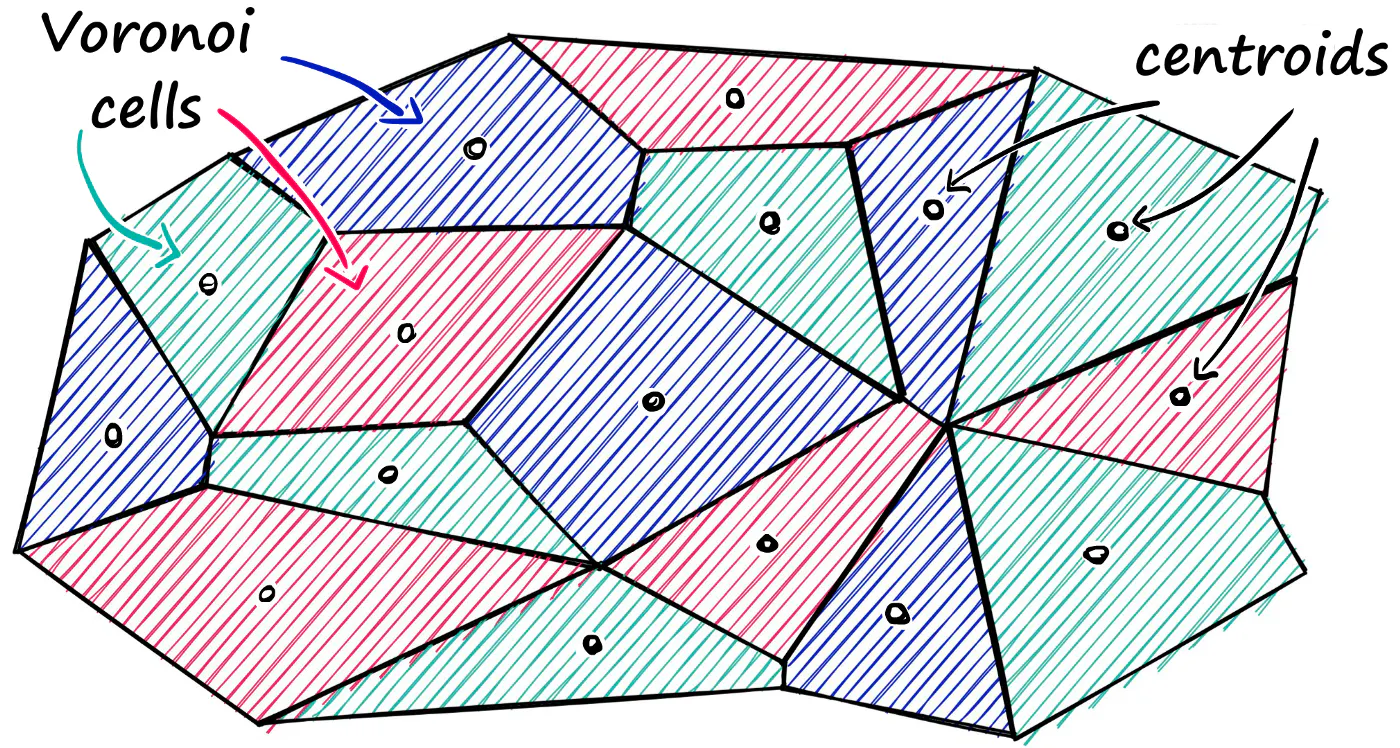

进行聚类的结果，一方面可以极大提升查询速度，但另一方面，可能会造成落在聚类簇边缘的“query向量”只在本聚类簇内查找匹配的结果（实际上，它可能与邻近的聚类簇的其他向量更靠近），从而导致匹配质量的降低。 一个缓解这个问题的方法是：调整参数 nprobe. 通过增加 nprobe (增加用于匹配查询向量的邻近聚类簇数量）来提升匹配质量。（同时，也会增加查询耗时）

Image credit: pinecone.io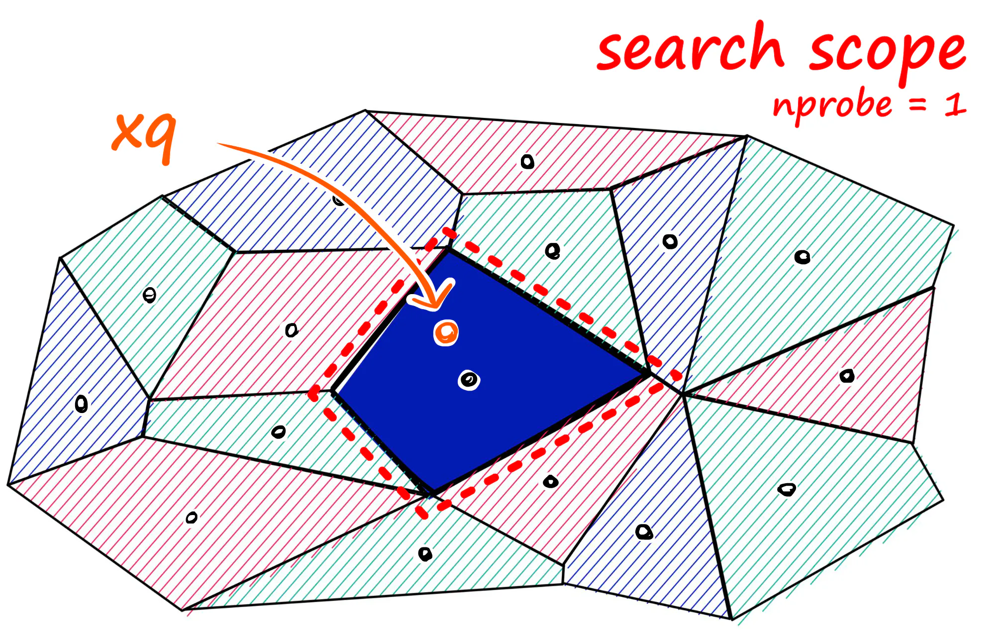

# Product Quantization

All of our indexes so far have stored our vectors as full (eg Flat) vectors. Now, in very large datasets this can quickly become a problem. Fortunately, Faiss comes with the ability to compress our vectors using Product Quantization (PQ). But, what is PQ? Well, we can view it as an additional approximation step with a similar outcome to our use of IVF. Where IVF allowed us to approximate by reducing the scope of our search, PQ approximates the distance/similarity calculation instead. PQ achieves this approximated similarity operation by compressing the vectors themselves, which consists of three steps.

1. Original vector
2. Sliced sub-vector
3. slice clustering
4. centroid ID vector

PQ（乘积量化）不是对嵌入向量空间进行降维，而是对向量本身进行压缩：

• 01 向量分段，例如：1024 -> 128x8 (8个片段)；
• 02 如果数据量是50k，则从单个50k x 1024 的矩阵，变成 8个 50k x 128 的矩阵；
• 03 然后分别用k=256的k-means进行聚类，得到8组256个centroids；则每个原始向量可以用长度为8的向量进行表征（8组与各个向量片段最近的centroid的ID）；
• 04 查询向量（query）同样进行片段化，并找到各组的centroids，然后计算片段向量与centroid的距离，并保存为距离表（partial query subvector-to-centroid distances table)；
• 05 查询向量与数据向量的距离？将数据向量的centroid-ID向量，用于 partial-query-distance-table 的表查询（table lookup），就能得到对应的一系列距离，然后计算其总和L2距离；
• 06 将查询向量与所有数据向量的距离计算出来，排序，即可得到 top-k 最近距离，亦即 top-k 最近似结果 （实际就是 KNN 算法）。
• 07 进一步的优化查询耗时，就是在计算距离的时候，不是对所有数据向量，而是只针对局部数据向量进行计算（也就是 IVF + PQ）。

Image credit: pinecone.io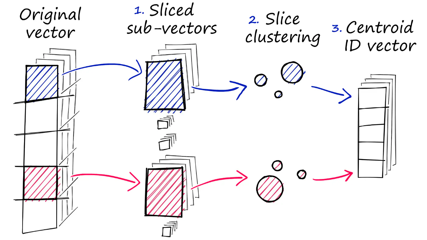

# Show me the code

 0
 1
 2
 3
 4
 5
 6
 7
 8
 9
10
11
12
13
14
15
16
17
18
19
20
21

import faiss  # here's the 'faiss-cpu' package actually

m = 8  # number of centroid IDs in final compressed vectors
bits = 8 # number of bits in each centroid
nlist = 50  # how many cells/blocks

# we keep the same L2 distance flat index
quantizer = faiss.IndexFlatL2(d)
index = faiss.IndexIVFPQ(quantizer, d, nlist, m, bits)

# sentence_embeddings:
# the target embeddings data from embedding model such as BERT/RoBERTa (or sentence-transformers)
index.train(sentence_embeddings)
index.add(sentence_embeddings)

index.nprobe = 10  # see the "IVF" part mention before

# xq: the query text
D, I = index.search(xq, k)  # searching top-k most similar vectors

for i in I.tolist()[0]:
    print(indata[i])  # indata: sample of original texts/sentences

# Example 01: 平凡的世界

0
1
2
3
4
5
6
7
8

d = sent_embeddings.shape[1]
nlist = 50  # how many cells
quantizer = faiss.IndexFlatL2(d)
index = faiss.IndexIVFFlat(quantizer, d, nlist)
k = 4
xq = embedding_model.encode(["秀莲的老家在哪里？"])
D, I = index.search(xq, k)
for i in I.tolist()[0]:
    print(indata[i])

01 她干脆给家里人说：周围没她看上的男人！她姐夫对她开玩笑说：“那到外地给你瞅个女婿！”她却认真地说：“只要有合心的，山南海北我都愿意去！爸爸暂时有你们照顾，将来我再把他接走……”家里人吃惊之余，又看她这样认真，就向他们所有在门外的亲戚和熟人委托，让这些人给他们的秀莲在外地寻个对象……本来秀莲只是随便这么说说；她并没指望真能在外地找个合适的男人。

02 这家不能分！你也不要担心秀莲会怎样，总有我哩！”“你千万不要怪罪秀莲！秀莲实在是个好娃娃！人家从山西过来，不嫌咱家穷，几年来和一大家人搅在一起。

03 秀莲有时就体贴地坐在她身边，给她背上搔痒痒，或者把她的几绺稀疏的白发理顺，在脑后挽成核桃大一个大发髻，老太太不时用她的瘦手，满怀深情地在秀莲身上抚摸着。

04 直到寒露过了十来天，贺耀宗从山西心焦地写信问秀莲怎还不回来？是不是病了？秀莲这才决定动身回家去。

# Example 02: 平凡的世界

 0
 1
 2
 3
 4
 5
 6
 7
 8
 9
10

d = sent_embeddings.shape[1]  # embedding's dimension
m = 8  # number of centroid IDs in final compressed vectors
bits = 8 # number of bits in each centroid
nlist = 50  # how many cells/blocks
quantizer = faiss.IndexFlatL2(d)
index = faiss.IndexIVFPQ(quantizer, d, nlist, m, bits)
k = 4
xq = embedding_model.encode(["秀莲的老家在哪里？"])
D, I = index.search(xq, k)
for i in I.tolist()[0]:
    print(indata[i])

01 “如果把家分开，咱就是烧砖也能捎带种了自己的地！就是顾不上种地，把地荒了又怎样？咱拿钱买粮吃！三口人一年能吃多少？”其实，这话才是秀莲要表达的最本质的意思。

02 分家其实很简单，只是宣布今后他们将在经济上实行“独立核算”，原来的家产少安什么也没要，只是秀莲到新修建起的地方另起炉灶过日月罢了。

03 秀莲五岁上失去母亲以后，一直是她父亲把她和她姐秀英拉扯大的。

04 她干脆给家里人说：周围没她看上的男人！她姐夫对她开玩笑说：“那到外地给你瞅个女婿！”她却认真地说：“只要有合心的，山南海北我都愿意去！爸爸暂时有你们照顾，将来我再把他接走……”家里人吃惊之余，又看她这样认真，就向他们所有在门外的亲戚和熟人委托，让这些人给他们的秀莲在外地寻个对象……本来秀莲只是随便这么说说；她并没指望真能在外地找个合适的男人。

单从这两个例子对比着看，个人感觉 indexIVFFlat() 的检索结果 (Example 01) 要优于 indexIVFPQ() 的检索结果 (Example 02)。

怎么简单的方法效果比高明的算法要好？这不对吧？这里其实是想说明一个观点：理论上的“较优”，通常都要针对一个广泛的统计结果而言。而这里只有两个例子，不能说明问题！

# index.range_search()

简而言之：range_search() 捞回射程半径内（threshold控制）的所有近邻。因此不同的 query_vector 可能会得到不同长度的返回结果，从而需要特别处理。

The method range_search returns all vectors within a radius around the query point (as opposed to the k nearest ones). Since the result lists for each query are of different sizes, it must be handled specially:

in C++ it returns the results in a pre-allocated RangeSearchResult structure

in Python, the results are returned as a triplet of 1D arrays lims, D, I, where
result for query i is in I[lims[i]:lims[i+1]] (indices of neighbors), D[lims[i]:
lims[i+1]] (distances).

Supported by (CPU only): IndexFlat, IndexIVFFlat, IndexScalarQuantizer, IndexIVFScalarQuantizer.

from official doc

NOTE that this may not be the latest info.

Example code block:

 0
 1
 2
 3
 4
 5
 6
 7
 8
 9
10
11
12
13
14
15
16
17
18
19
20
21
22
23
24
25
26
27
28
29
30
31
32
33
34
35

# read the text data, and get the embeddings:
#texts_data = pd.Series(...)
#sentence_embeddings = embedding_model.encode(texts_data.values)


# First, you need to use an index that supports Inner Product as metric, for example :
d = sentence_embeddings.shape[1]

nlist = 10  # how many voronoi cells
quantizer = faiss.IndexFlatL2(d)
index = faiss.IndexIVFFlat(quantizer, d, nlist)

index.train(sentence_embeddings)
index.add(sentence_embeddings)

query = ["there and back again", "a hobbit's journey"]
xq = embedding_model.encode(query)

# Then, you should probably normalize all embeddings first
# ( the inner product between two normalized embeddings corresponds to their cosine similarity )
# https://github.com/facebookresearch/faiss/blob/master/python/faiss.py#L673
faiss.normalize_L2(x=sentence_embeddings)
faiss.normalize_L2(x=xq)

threshold = 0.95
lims, D, I = index.range_search(x=xq, thresh=threshold)

# turn search results into dataframes
dfresults = []
for i in range(len(xq)):
    Ii = I[lims[i]:lims[i+1]]
    Di = D[lims[i]:lims[i+1]]
    dfout = pd.concat([texts_data[Ii], pd.Series(Di, index=Ii)], axis=1)
    dfout.columns = ["texts", "distances"]
    dfresults.append(dfout)